Introduction
- Production is the process by which inputs are transformed into ‘output’. Production is carried out by production or firms. A firm acquires different inputs like labour, machines, land, raw materials etc. it uses these inputs to produce output. This output can be consumed by consumers, or used by other firms for further production. For example, a tailor uses a sewing machine, cloth, thread and his own labour to ‘produce’ shirts. A farmer uses his land, labour, a tractor seed, fertilizer, water etc to produce wheat.
- In order to acquire inputs a firm has to pay for them. This is called the cost of production. Once output has been produced, the firm sell it in the market and earns revenue. The difference between the revenue and cost is called the firm’s profit.
Production Function
The production function of a firm is a relationship between inputs used and output produced by the firm. For various quantities of inputs used, we assume that the farmer uses only two inputs to produce wheat : land and labour. A production function tells us the maximum amount of wheat he can produce for a given amount of land that he uses, and a given number of hours of labour that he performs. Suppose that he uses 2 hours of labour/day and 1 hectare of land to produce a maximum of 2 tonnes of wheat. Then, a function that describes this relation is called a production function.
One possible example of the form this could take is:
Q = K X L,
Where, q is the amount of wheat produced, K is the area of land in hectares, L is the number of hours of work done in a day.
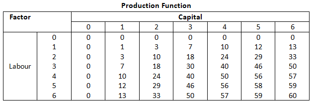
A numerical example of production function is given. The left column shows the amount of labour and the top row shows the amount of capital. As we move to the right along any row, capital increases and we move down along any column, labour increases. For different values of the two factors, the table shows the corresponding output levels. For example, with 1 unit of labour and 1 unit of capital, the firm can produce at most 1 unit of output; with 2 units of labour and 2 units of capital, it can produce at most 10 units of output; with 3 units of labour and 2 units of capital, it can produce at most 18 units of output and so on. In our example, both the inputs are necessary for the production. If any of the inputs becomes zero, there will be no production. With both inputs positive output will be positive. As we increase the amount of any input, output increases.
The Short Run and The Long Run
The short run – The short run, at least one of the factor – labour on capital – cannot be varied, and therefore, remains fixed. In order to vary the output level, the firm can vary only the other factor. The factor that remains fixed is called the fixed factor whereas the other factor which the firm can vary is called the variable factor. Consider the example represented through. Suppose, in the short run, capital remains fixed at 4 units. Then the corresponding column shows the difference levels of output that the firm may produce using different quantities of labour in the short run.
The long run – the long run, all factors of production can be varied. A firm in order to produce different levels of output in the long run may vary both the inputs simultaneously. So, in the long run, there is no fixed factor.
Total Product, Average Product and Marginal Product
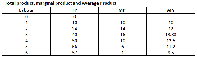
Total Product – Suppose we very a single input and keep all other inputs constant. Then for different levels of that input, we get different levels of output. This relationship between the variable input and output, keeping all other inputs constant, is often referred to as of the variable input.
Average Product – Average product is defined as the output per unit of variable input. We calculate it as
APL = TPL/L
The last column of gives us numerical example of average product of laobur for the production function described. Values in this column are obtained by dividing TP by L.
Marginal Product – Marginal product of an input is defined as the change in output per unit of change in the input when all other inputs are held constant. When capital is held constant, the marginal product of labour is
MPL = Change in output / change in input
= ΔTPL /ΔL
Where Δ represent the change of the variable.
Average product of an input at any level of employment is the average of all marginal products up to that level. Average and marginal products are often referred to as average and marginal returns, respectively, to the variable input.
The law of diminishing marginal product and the law of variable proportions
if we plot the data on graph paper, placing laobur on the X-axis and output on the Y-axis, we get the curve shown in the diagram below, Let us examine what is happening to TP. Notice that TP increases as labour input increases. But the rate at which it increases in not constant. An increase in labour from 1 to 2 increases. TP by 10 units. An increase in labor from 2 to 3 increases TP by 12. The rate at which TP increases, as explained above is shown by the MP. Notice the MR first increases and the begins to fall. This tendency of the MP to first increases and then fall is called the law of variable proportions or the law of diminishing marginal product. Law of variable proportions say that the marginal product of a factor input initially rises with its employment level.
Shapes of total product, marginal product and average product curves
An increase in the amount of one of the inputs keeping all other inputs constant results in an increase in output. How the total product changes as the amount of labour increases. The total product curve in the input-output plane is a positively sloped curve. The shape of the total product curve for a typical firm. We measure units of laobur along the horizontal axis and output along the vertical axis. With L units of labour, the firm can at most produce q1 units of output. According to the law of variable proportions, the marginal product of an input initially rises and then after a certain level of employment, it starts falling. The MP curve therefor, looks like an inverse ‘U’ shaped curves.
Returns to Scale – The law of variable proportions arises because factor proportions change as long as one factor is held constant and the other is increased. What if both factors can change? Remember that this can happen only in the long run. One special case in the long run occurs when both factors are increased by the some proportion, or factors are scaled up.
When a proportional increase in all inputs results in an increase in output by larger proportion, the production function is said to display increasing returns to scale (IRS)
Decreasing Returns to Scale (DRS) holds when a proportional increase in all inputs results in an increase in output by a smaller proportion. For example, suppose in a production process, all input get doubled. As a result, if the output gets doubled, the production function exhibits CRS. If outputs is less than doubled, then DRS holds, and if it is more than doubled, then IRS holds.
Costs –
- In order to produce output, the firm needs to employ inputs. But a given level of output, typically, can be produced in many ways.
- There can be more than one input combinations with which a firm can produce a desired level of output.
- We can see that 50 units of output can be produced by three different input combinations (L = 6, K = 3), (L = 4, K = 4) and (L = 3, K = 6).
- The questions is which input combination will the firm choose? With the input prices given, it will choose that combination of inputs which is least expensive.
- So, for every level of output, the firm chooses the least cost input combination.
- Thus the cost function describes the least cost of producing each level of output given prices of factors of production and technology.
- Short run costs – In the short run, some of the factors fo production cannot be varied, and therefore, remain fixed. The cost that a firm incurs to employ these fixed inputs is called the total fixed cost (TFC). Whatever amount of output the firm produces, this cost remains fixed for the firm. To produce any required level of output, the firm, in the short run, can adjust only variable inputs. Accordingly, the cost that a firm incurs to employ these variable inputs is called the total variable cost (TVC). Adding the fixed and the variable costs, we get the total cost (TC) of a firm
TC = TVC + TFC
- Short run average cost (SAC) – incurred by the firm is defined as the total cost per unit of output. We calculate it as
SAC = TC/q
- Average variable cost (AVC) – is defined as the total variable cost per unit of output. We calculate it as
AVC = TVC/q
Average fixed cost (AFC) is
AFC = TFC/q
- Short run marginal cost (SMC) – is defined as the change in total cost per unit of change in output
SMC = change in total cost / change in output
= ΔTC / Δq
Shapes of the short Run Cost Curves – now let us see what these short run cost curves look like. You could plot the data from placing output on the x-axis and costs on the y-axis.
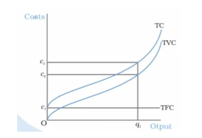
Cost. These are total fixed cost (TFC), total variable cost (TVC) and total cost (TC) curves for a firm. Total cost is the vertical sum of total fixed cost and total variable cost.
Figure 3.3 illustrates the shapes of total fixed cost, total variable cost and total cost curves for a typical firm. We place output on the x-axis and costs on the y-axis. TFC is a constant which takes the value C1 and does not change with the change in output. It is, therefore, a horizontal straight line cutting the cost axis at the point C1. At q1, TVC is C2 and TC is C3.
Show the shape of average fixed cost curve for a typical firm. We measure output along the horizontal axis and AFC along the vertical axis. At q1 level of output, we get the corresponding average fixed cost at F. The TFC can be calculated as
TFC = AFC x quantity
= OF x Oq1
= the area of the rectangle OFCq1
Long Run Costs –
In the long run, all inputs are variable. There are no fixed costs. The total cost and the total variable cost therefore, coincide in the long run. Long run average cost (LRAC) is defined as cost per unit of output, i.e.
LRAC = TC/q
Long run marginal cost (LRMC) is the change in total cost per unit of change, in output. When output changes in discrete units, then, if we increase production from q1 – 1 to q1 units of output, the marginal cost of producing q1th unit will be measured as
LRMC = (TC at q1 units) – (TC at q1 – 1 units)
Just like the short run, in the long run, the sum of all marginal costs up to some output level gives us the total cost at that level.
Shapes of the Long Run Cost Curves – IRS implies that if we increase all the inputs by a certain proportion, output increases by more than that proportion.
DRS implies that if we want to increase the output by a certain proportion, inputs need to by increased by more than that proportion. As a result, cost also increase by more than proportion. So, as long as DRS operates, the average cost must be rising as the firm increases output.
CRS implies a proportional increase in inputs resulting in a proportional increase in output. So the average cost remains constant as long as CRS operates.