Utility – A consumer usually decides his demand for a commodity on the basis of utility (or satisfaction) that he derives from it. Utility of a commodity is its want-satisfying capacity. The more the need of a commodity or the stronger the desire to have it. The greater is the utility derived from the commodity.
Utility is subjective. Different individuals can get different levels of utility from the same commodity. For example, some one who likes chocolates will get much higher utility from a chocolate than some one who is not so fond of chocolates.
Cardinal Utility Analysis – Cardinal utility analysis assumes that level of utility can be expressed in numbers. For example, we can measure the utility derived from a shirt and say, this shirt gives me 50 units of utility. Before discussion further, it will be useful to have look at two important measures of utility.
Measures of Utility
- Total Utility – Total utility of a fixed quantity of a commodity (TU) is the total satisfaction derived from consuming the given amount of some commodity x. More of commodity x provides more satisfaction to the consumer. TU depends on the quantity of the commodity consumed. Therefore, TU refers to total utility derived from consuming n units of a commodity x.
- Marginal Utility – Marginal utility (MU) is the change in total utility due to consumption of one additional unit of a commodity. For example, suppose 4 bananas give us 28 units of total utility and 5 bananas give us 30 units of total utility.
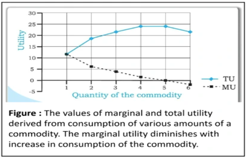
Values of marginal and total utility derived from consumption of various amounts of a commodity
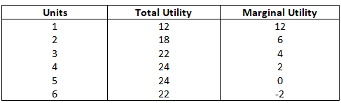
Notice that MU3 is less than MU2. You may also notice that total utility increases but at a diminishing rate: The rate of change in total utility due to change in quantity or commodity consumed is a measure of marginal utility. This marginal utility diminishes with increase in consumption of the commodity from 12 to 6, 6 to 4 and so on. This follows from the law of diminishing marginal utility. Low of Diminishing Marginal Utility states that marginal utility from consuming each additional unit of a commodity declines as its consumption increases, while keeping consumption of other commodities constant.
Derivation of Demand Curve in the Case of a Single Commodity (Law of Diminishing Marginal Utility)
- Cardinal utility analysis can be used to derive demand curve for a commodity. What is demand and what is demand curve? The quantity of a commodity that a consumer is willing to buy and is able to afford, given prices of goods and income of the consumer, is called demand for that commodity.
- Demand for a commodity x, apart from the price of x itself, depends on factors such as prices of other commodities (see substitutes and complements 2.4.4), income of the consumer and tastes and preferences of the consumers.
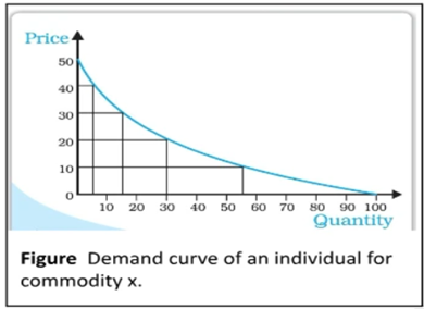
- Demand curve is a graphic presentation of various quantities of a commodity that a consumer is willing to buy at different prices of the same commodity, while holding constant prices of other related commodities and income of the consumer.
The downward sloping demand curve shows that at lower prices, the individual is willing to buy more of commodity x, at higher prices, she is willing to buy less of commodity x. therefore, there is a negative relationship between price of a commodity and quantity demanded which is referred to as the Law of Demand.
Ordinal Utility Analysis –
Cardinal utility analysis is simple to understand, but suffers from a major drawback in the form of quantification of utility in numbers. In real life, we never express utility in the form of numbers. At the most, we can rank various alternative combinations in terms of having more or less utility. In other words, the consumer does not measure utility in numbers, though she often ranks various consumption bundles. This forms the starting point of this topic – ordinal Utility Analysis.
Definition of Indifference Curve
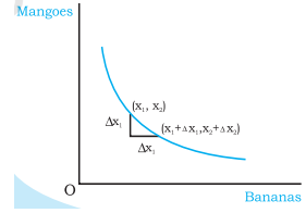
An indifference curve is the curve which represents all those combinations of two commodities which give the same level of satisfaction to a consumer. It slopes downward because an increase in the amount of good 1 along the indifference curve is associated with a decrease in the amount of goods 2 as the preferences are monotonic. Marginal Rate of Substitution (MRS) means the rate at which the consumer is willing to substitute one commodity for the other commodity.
MRSxy = Quantity of the good sacrificed / Quantity of the good obtained.
Feature of Indifference Curve
- Indifference curve slopes downwards from left to right – An indifference curve slopes downwards from left to right, which means that in order to have more of bananas, the consumer has to forgo some mangoes. It the consumer does not forego some mangoes with an increase in number of bananas, it will mean consumer having more of bananas with same number of mangoes, taking her to a higher indifference curve. Thus, as long as the consumer is on the same indifference curve, an increase in bananas must be compensated by a fall in quantity of mangoes.
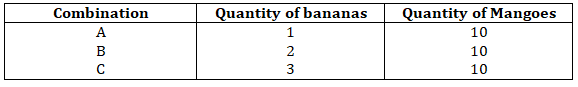
2. Higher indifference curve gives greater level of utility – As long as marginal utility of a commodity is positive, an individual will always prefer more of that commodity, as more of the commodity will increases the level of satisfaction.
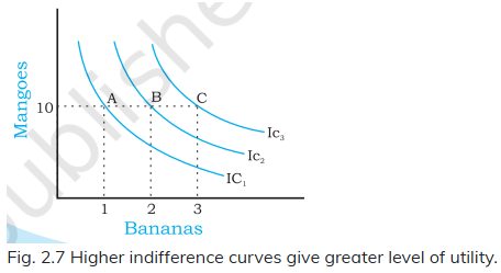
Representation of different level of utilities from different combination of goods
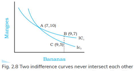
3. Two indifference curve never interest each other – Two indifference curves intersecting each other will lend to conflicting results. To explain this, let us allow two indifference curves to intersect each other as shown. As points A and B lie on the same indifference curve IC1, utilities derived from combination A and combination B will give the same level of satisfaction. Similarly, as points A and C lie on the same indifference curve IC2, utility derived from combination A and from combination C will give the same level of satisfaction.
The Consumer’s Budget – Let us consider a consumer who has only a fixed amount of money (income) to spend on two goods. The prices of the goods are given in the market. The consumer cannot buy any and every combination of the two goods that she may want to consume. The consumption bundles that are available to the consumer depend on the prices of the two goods and the income of the consumer.
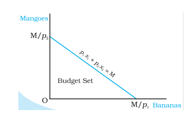
Budget Set and Budget Line – Suppose the income of the consumer is M and the prices of bananas and mangoes are p1 and p2 respectively. It the consumer wants to buy x1 quantities of bananas, she will have to spend p1x1 amount of money. Similarly, if the consumer wants to buy x2 quantities of mangoes, she will have to spend p2x2 amount of money. The set of bundles available to the consumer is called the budget set.
Example – Consider, for example, a consumer who has Rs.20, and suppose, both the goods are priced at Rs.5 and are available only in integral units.
If both the goods are perfectly divisible, the consumer’s budget set would consist of all bundles (X1, X2) such that X1 and X2 are nay numbers greater than or equal to 0 and P1X1+P2X2 ≤ M. The budget set can be represented in a diagram. All bundles in the positive quadrant which are on or below the line are included in budget set. The equation of the line is
P1X1 + P2X2 = M
The line consists of all bundles which cost exactly equal to M. This line is called the budget line.
Changes in the Budget Set – The set of available bundles depends on the prices of the two goods and the income of the consumer. When the price of either of the goods or the consumer’s income changes, the set of available bundles is also likely to change. Suppose the consumer’s income changes from M to M’ but the prices of the two goods remain unchanged. With the new income, the consumer can afford to buy all bundles (X1, X2) such that P1X1 + P2X2 ≤ M’. Now the equation of the budget line is
P1X1 + P2X2 ≤ M’
Equation can also be written as
X2 = M’/P2 – P1/P2 X1
Note that the slope of the new budget line is the same as the slope of the budget line prior to the change in the consumer’s income. However, the vertical intercept has changes after the change in income. It there is an increase in the income, i.e. if M’>M, the vertical as well as horizontal intercepts increase, there is a parallel outward shift of the budget line. If the income increases, the consumer can buy more of the goods at the prevailing market prices. Similarly, if the income goes down, i.e. if M’<M, both intercepts decrease, and hence, there is a parallel inward shift of the budget line. If income goes down, the availability of goods goes down. Changes in the set of available bundles resulting from changes in consumer’s income when the prices of the two goods remain unchanged.
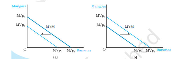
Changes in the Set of Available Bundles of Goods Resulting from changes in the consumer’s income. A decrease in income causes a parallel inwards shift of the budget line as in panel (a). An increase in income causes a parallel outward shift of the budget line as in panel (b).
Optimal Choice of The Consumer
In economics, it is assumed that the consumer chooses her consumption bundle on the basis of her tatse and preferences over the bundles in the budget set. It is generally assumed that the consumer has well defined preferences over the set of all possible bundles. She can compare any two bundles. In other words, between any two bundles, she either prefers one to the other or she is indifferent between the two.
In economics, it is generally assumed that the consumer is a rational individual. A rational individual clearly knows what is good or what is bad for her, and in any given situation, she always tries to achieve the best for herself. Thus, not only does a consumer have well-defined preference over the set of available bundles, she also acts according to her preferences. From the bundles which are available to her, a rational consumer always chooses the one which gives her maximum satisfaction.
Illustrates the consumer’s optimum. At (X1,X2), the budget line is tangent to the black coloured indifference curve. The first thing to note is that the indifference curve just
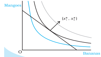
touching the budget line is the highest possible indifference curve given the consumers’ budget set. Bundles on the indifference curves above this, like the grey one, are not affordable. Points on the indifference curves below this, like the blue one, are certainly inferior to the points on the indifference curve, just touching the budget line. Any other point on the budget line lies on a lower indifference curve and hence, is inferior to (X1,X2) . Therefore, (X1,X2) is the consumer’s optimum bundle.
Demand
The quantity of a commodity that a consumer is willing to buy and is able to afford, given prices of goods and consumer’s tastes and preferences is called demand for the commodity. Whenever one or more of these variables change, the quantity of the good chosen by the consumer is likely to change as well. Here we shall change one of these variables at a time and study how the amount of the good chosen by the consumer is related to that variable.
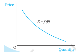
Demand curve. The demand curve is a relation between the quantity of the good chosen by a consumer and the price of the good. The independent variable (price) is measured along the veritable (price) is measured along the vertical axis and dependent variable (quantity) is measured along the horizontal axis. The demand curve gives the quantity demanded by the consumer at each price.
Demand Curve and the Law of Demand – If the prices of other goods, the consumer’s income and her tastes and preferences remain unchanged, the amount of good that the consumer optimally chooses, becomes entirely dependent on its price. The relation between the consumer’s optimal choice of the quantity of a good and its price is very important and this relation is called the demand function.
Deriving a Demand Curve from Indifference Curves and Budget Constraints – Consider an individual consuming bananas (X1) and mangoes (X2), whose income is M and market prices of X1 and X2 are P’1 and P’2 respectively. Figure (a) depicts her consumption equilibrium at point C, where buys X’1 and X’2 quantities of bananas and mangoes respectively. In panel (b) of figure 2.14, we plot P’1 against X’1 which is the first point on the demand curve for X1.
The negative slope of the demand curve can also be explained in terms of two effects namely, substitution effect and income effect that come into play when price of a commodity changes. When bananas become cheaper, the consumer maximises his utility by substitution bananas for magnoes in order to derive the same level of satisfaction of a price change, resulting in an increase in demand for bananas.
Moreover, as price of bananas drops, consumer’s purchasing power increases, which further increases demand for bananas (and mangoes). This is the income effect of a price change, resulting in further increase in demand for bananas.
Law of Demand – Law of Demand states that other thing being equal, there is a negative relation between demand for a commodity and its price. In other words, when price of the commodity decreases, demand for it rises, other factors remaining the same.
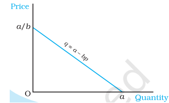
Linear Demand – A linear demand curve can be written as
D(p) = a – bp; 0 ≤ p ≤ a/b
= 0; p > a/b
Where a is the vertical intercept, -b is the shop of the demand curve. At price 0, the demand is a, and at price equal to a/b, the demand is 0. The slope of the demand curve measures the rate at which demand changes with respect to its price. For a unit increase in the price of the good, the demand falls by b units.
Normal and Inferior Goods – The quantity of good that the consumer demands can increase or decrease with the rise in income depending on the nature of the good. For most goods, the quantity that a consumer choose, increases as the consumer’s income increases and decreases as the consumer’s income decreases. Such goods are called normal goods. Thus, a consumer’s demand for a normal good moves in the same direction as the income of the consumer. However, there are some goods the demands fro which mover in the opposite direction of the income of the consumer. Such goods are called inferior goods.
Substitute’s and Complements –
- We can also study the relation between the quantity of a good that a consumer chooses and the price of a related good.
- The quantity of a good that the consumer chooses can increase or decrease with the rise in the price of a related good depending on whether the two goods are substitutes or complementary to each other.
- Goods which are consumed together are called complementary goods. Examples of goods which are complement to each other include tea and sugar, shoes and socks, pen and ink, etc. Since tea and sugar are used together, an increase in the price of sugar is likely to decrease the demand for tea and a decrease in the price of sugar is likely to increase the demand for tea.
- Similar is the case with other complements. In general, the demand for a good moves in the opposite direction of the price of its complementary goods.
Shifts in the Demand Curve
The demand curve was drawn under the assumption that the consumer’s income, the price of other goods and the preferences of the consumer are given. What happens to the demand curve when any of these things changes? Given the prices of other goods and the preferences of a consumer, if the income increases, the demand for the good at each price changes, and hence, there is a shift in the demand curve. For normal goods, the demand curve shifts rightward and for inferior goods, the demand curve shifts leftward.
Given the consumer’s income and her preferences, if the price of a related good changes, the demand for a good at each level of its price changes, and hence, there is a shift in the demand for a good at each level of its price changes, and hence, there is a shift in the demand curve. If there is an increase in the price of a substitute good, the demand curve. If there is an increase in the price of a substitute good, the demand curve shifts rightward. On the other hand, if there is an increase in the price of a complementary good, the demand curve shifts leftward.
Movements along the demand curve and shifts in the Demand curve
As it has been noted earlier, the amount of a good that the consumer chooses depends on the price of the good, the prices of other goods, income of the consumer and her tastes and preferences. The demand function is a relation between the amount of the good and its price when other things remain unchanged. The demand curve is a graphical representation of the demand function. At higher prices, the demand is less, and at lower prices, the demand is more. Thus, any change in the price leads to movements along the demand curve. On the other hand, changes in any of the other things lead to a shift in the demand curve. A movement along the demand curve and a shift in the demand curve.
Market Demand – In the last section, we studied the choice problem of the individual consumer and derived the demand curve of the consumer. However, in the market for a good, there are many consumers. It is important to find out the market demand for the good. The market demand for a good at a particular price is the total demand of all consumers taken together. The market demand for a good can be derived from the individual demand curves. Suppose there are only two consumers in the market for a good.
Elasticity of Demand – The demand for a good moves in the opposite direction of its price. But the impact of the price change in always not the same. Sometimes, the demand for a good changes considerably even for small price changes. On the other hand, there are some goods for which the demand is not affected much by price changes. Demands for some goods are very responsive to price changes while demands for certain other are not so responsive to price changes. Price elasticity of demand is a measure of the responsiveness of the demand for a good to changes in its price. Price elasticity of demand for a good is defined as the percentage change in demand for the good divided by the percentage change in its price. Price-elasticity of demand for a good
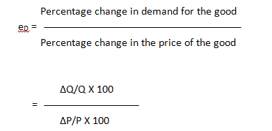
Where, ΔP is the change in price of the good and ΔQ is the change in quantity of the good.
Example – Suppose an individual buy 15 bananas when its price is Rs.5 per banana. When the price increase to Rs.7 per banana, she reduces his demand to 12 bananas.
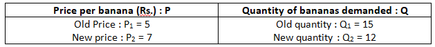
In order to find her elasticity demand for bananas, we find the percentage change in quantity demanded and its price, using the information summarized in table.
Note that the price elasticity of demand is a negative number since the demand for a good is negatively related to the price of a good. However, for simplicity, we will always refer to the absolute value of the elasticity.
Percentage change in quantity demanded = ΔQ/Q1x100
= (Q2 – Q1/Q1)x100
= 12 -15/15 x100
= -20
Percentage change in Market Price = ΔP/P1 x 100
= (P2 – P1/P1)x 100
= 7 – 5 / 5 x 100
= 40
Elasticity along a Linear Demand Curve –
Let us consider a linear demand curve q = a – bp. Note that at any point on the demand curve, the change in demand per unit change in the price Δq/Δp = -b.
Substituting the value of Δq / Δp in (2.16b)
We obtain, eD = – b x p/q
ED = – bp/a – bp
It is clear that the elasticity of demand is different at different points on a liner demand curve. At p = 0, the elasticity is 0, at q = 0, elasticity is ꚙ. At = p = a /2b, the elasticity is 1, at any price greater than o and less than a/2b, elasticity is less than 1, and at any price greater than q/2b, elasticity is greater than 1. The price elasticity’s of demand along the linear demand curve given by equation are depicted.
Constant Elasticity Demand Curve – The elasticity of demand on different points on a linear demand curve is different varying from 0 to ꚙ. But sometimes, the demand curves can be such that the elasticity of demand remains constant throughout. Consider, for example, a vertical demand curve as the one depicted. Whatever be the price, the demand is given at the level q. A price never leads to a change in the demand for such a demand curve and |eD| is always 0. Therefore, a vertical demand curve is perfectly inelastic.
Factors Determining Price Elasticity of Demand for a good
The price elasticity of demand for a good depends on the nature of the good and the availability of close substitutes of the good. Consider, for example, necessities like food. Such goods are essential for life and the demands for such goods do not change much in response to change in their prices. Demand for food does not change much even if food prices go up. On the other hand, demand for luxuries can be very responsive to price changes. In general, demand for a necessity is lidley to be price inelastic while demand for a luxury good is likely to be price elastic.
Elasticity and Expenditure – The expenditure on a good is equal to the demand for the good times its price. Often it is important to know how the expenditure on a good changes as a result of a price change. The price of a good and the demand for the good are inversely related to each other. Whether the expenditure on the good goes up or down as result fo an increase in its price depends on how responsive the demand for the good is to the price change.
Consider an increase in the price of a good. If the percentage decline in quantity is greater thatn the percentage increase in the price, the expenditure on the good will go down.
Now consider a decline in the price of the good. If the percentage increase in quantity is greater than the percentage decline in the price, the expenditure on the good will go up. The expenditure on the good would change in the opposite direction as the price change if and only if the percentage change in quantity is greater than the percentage change in price, ie if the good is price-elastic. The expenditure on the good would change in the same direction as the price change if and only if the percentage change in quantity is less than the percentage change in price, i.e., if the good is price inelastic.