4. Organisation of Data

Meaning of Classification –

Classification is the process of arranging data into sequences and groups according to their common characteristics or separating them into different but related parts.

The given definition by Professor Connor highlights two important features of classification:

• Grouping on the basis of similarities – Classification arranges items into groups according to common resemblances and affinities. For example – in a library, books are grouped as Sciences, Literature, Commerce, etc.
• Grouping on the basis of unity in diversity – Even though individuals are diverse, classification expresses the unity of common attributes among them. For example – students in a class may differ in height, weight, or habits, but they can be grouped by age (e.g., 15 years old, 16 years old, etc.).

Objectives of Classification

The main objectives of classification are:

1. To simplify and condense the mass of data – In classification, the aim is to eliminate unnecessary details and convert the huge mass of complex data in to simple, condensed, logical & comprehensible form. It helps in highlighting the significant features of the data. For example – the huge and fragmented data collected during a population census has to be classified according to sex, marital status, education, occupation, etc., to ascertain the structure and nature of the population.
2. To explain similarity and dissimilarity of Data – Classification facilitates the grouping of data according to certain similarities (affinities) and dissimilarities (diversities). This enables the investigators to grasp them easily. Facts like educated and uneducated, married and unmarried, employed and unemployed, etc. are kept in separate classes.
3. To facilitate comparisons – Classification enables us to make meaningful comparisons, draw inferences and locate fact.
4. To study the relationships – Classification helps in finding out cause and effect relationship based on some criteria between the data. For example – The characteristics of income and education can be related after classifying the mass of data.
5. To prepare the data for tabulation – Only classified data can be presented in tabular form classification, thus provides a basis for tabulation and further statistical processing.

Requisites of a Good Classification

A good classification must possess the following features:

1. Suitability – The classification should conform to the object of the enquiry. For example – if investigation is conducted to inquire into the economic condition of workers, then it will be of no use to classify them on basis their religion.
2. Unambiguous – The classification should not lead to any ambiguity or confusion. It should not be difficult to place units into different groups according to their common characteristics.
3. Exhaustiveness – Classification should be so exhaustive that every unit of the series should find place in one group or another.
4. Flexibility – A good classification should be capable of being adjusted according to the changed situations and conditions.
5. Mutually Exclusive – The classes must not overlap so that an observed value belongs to one and only one of the classes. There must be no item which can find its way into more than one class.

Methods of Classification

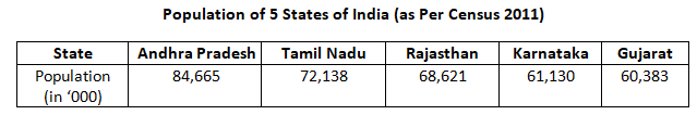
1. Geographical Classification (or Spatial Classification) – When the data is classification according to geographical location or region (such as countries, states, districts, etc.), it is known as geographical classification.

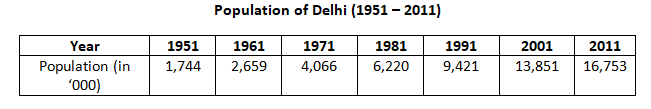
2. Chronological Classification (or Temporal Classification) – When data is classified with respect to different periods of time (such as decade, years, months, etc.), the type of classification is known as chronological classification.

3. Qualitative Classification – In qualitative classification, data is classification on the basis of descriptive characteristics or on the basis of attributes like sex, literacy, region, caste, education, etc. which cannot be quantified. Such characteristics are called qualities or Attributes.

This type of classification is of two types:

• Simple Classification – When facts are classified into two classes according to one attribute only, then the classification is said to be simple. For example – if we divide (or classify) the population of a city into two groups (males and females), then the classification is simple.
• Manifold Classification – When facts are classified according to more than one attribute, or when each class is sub-divided into more than two sub-classes, then the classification is said to be manifold. For example – If we classify the population of a city into males and females, then subdivide into literates and illiterate and further subdivide according to marital status, we find that a number of classes are formed.

4. Quantitative Classification (or Numerical Classification) – In this classification, data is classified on the basis of some characteristics which can be measured such as height, weight, income, expenditure, production, or sales.

Concept of Variable

A variable refers to quantity or characteristic whose value varies from one investigation to another.

• The difference in value may be with respect to individuals, items, places or time.
• Each value within such range is called a ‘Variate’.
• Example :

1. “Price” is a variable as prices of different commodities are different.
2. “Age” is a variable as age of different students varies.
3. Similarly, some more variables are: Height, Weight, Wages, Expenditure, Imports, Production, etc.

Variables are of two kinds:

1. Discrete Variable (Discontinuous Variable) – Variables which are capable of taking only exact or finite value and generally not any fractional value are termed as discrete variables. In other words, discrete variables are expressed in terms of complete numbers. For example – number of workers or number of students in a class are discrete variable as they cannot be in fractions. Similarly, number of members in a family can be 1,2, 3 or so on, but cannot be 1 ¼ , 1 ½ and so on. Some other examples can be population of a town.
2. Continuous Variable – Those variable which can take all the possible values (integral as well as fractional), in a given specified range are termed as continuous variable s. in  a case, data is obtained by measurement. For example – Weight of students is a continuous variable because it can be measured in any value in the range of measurement, like 57 kg, 57.1 kg, 57.25 kg, 57.37 kg and so on. In the given case, weights are grouped into intervals like 50-55 kg (10 students), 55-60 kg (5 students) and so on. Values like 57 kg, 57.1 kg, 57.25 kg, 57,37 kg lie within these intervals.

Statistical Series – The arrangement of classified data in some logical order, like according to the size, according to the time of occurrence or according to some other measurable or non-measurable characteristics, is known as Statistical Series.

• Statistical series are prepared to present the collected and classified data in a properly arranged way.
• For example – if data pertaining to marks of 35 students in a class are arranged according to their roll numbers in the ascending or descending order, then the data so arranged would be known as statistical series.

Statistical Series on the basis of Construction

Individual Series – Individual series refers to that series in which items are listed singly, i.e. each item is given a separate value of measurement. For example – if marks of 10 students in Class XI are given individually, it will form an individual series.

Types of Individual Series

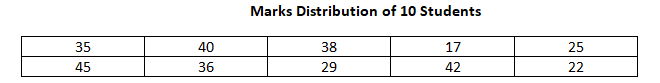
(i) Unorganized Individual Series (or Raw Data) – Unorganized series is an unarranged mass of data (raw data). Raw data means data in original form. When the investigator has collected the data and he not arranged the same in a systematic manner, it is called raw data or unorganized data. For example – Marks obtained by 10 students in a class are as follows:

(ii) Organized Individual Series – Organized series is an orderly arrangement of raw data. An organized individual series may be presented in two ways:

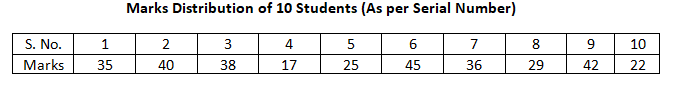
According to Serial Number – An individual series can be arranged in a serial order. So, marks obtained by 10 students may be arranged either in serial number or in order of their roll number as shown in the following table:

• According to order of Magnitude (Ascending or Descending order) – An individual series can also be arranged in order of magnitudes (ascending order or descending order).

>> The arrangement of raw data in ascending or descending order of magnitude is known as ‘Array’. It is also known as ‘Arrays’ or ‘Arraying of the data’ or ‘Arraying of the figures’.

Discrete Series (Or Frequency Array) – A discrete series is that series where individual values differ from each other by definite amount.

1. In a discrete series, various values of the variable are shown along with their corresponding frequencies.
2. For a discrete variable, the classification of its data is known as a ‘Frequency Array’.

Construction of Discrete Series using Tally Marks – The method of Tally Marks or Tally Bars is used to count the number of observations or the frequency of each value of the variable.

Important Terms –

1. Frequency – It refers to number of times a given value appears in a distribution. For example – suppose there are 20 students in a class and out of them, 9 students have got 70 marks, 6 got 85 marks, and 5 got 92 marks. Now, frequencies will be 9, 6, and 5 respectively.
2. Frequency Array – It refers to a series that shows the frequency corresponding to discrete values of a variable. A discrete variable can only take on a finite or countable number of values, like number of children, shoe size, etc.

Relative Frequency Distribution – When actual frequencies are expressed as a percentage of total number of observation, then relative frequencies are obtained.

Continuous Series (Grouped Frequency Distribution)

As compared to a discrete variable, a continuous variable can take any value in an interval. A continuous series is that series which represents continuous variables, showing range of values of different items of the series.

Important Terms under Continuous Series

1. Class – It hereby means a group of numbers in which items are placed such as 0 – 10, 10 -20, 20 – 30, etc.

• The classes should be clearly defined and should not lead to any confusion.
• Classes should be exhaustive, i.e. every value must fall into some class.

2. Class limits – The lowest and highest values of the variable within a class is called ‘class limit’. Each class is located between two number, which make class limit. The lowest value of a class is known as ‘lower limit’ or ‘I₁’ while the highest value is ‘upper limit’ or ‘I₂’. For example – in class 10 – 20 , lower limit (I₁) is 10 and upper limit (I₂) is 20.

3. Class – Interval (Class – Width) – The difference between the lower limit (I₁) and upper limit (I₂) of a class is known as class- interval. It is indicated by ‘I’ or ‘c’. Class – interval is also known as ‘magnitude’ or ‘size’ or ‘length’ of the class.

4. Range – The range of a frequency distribution can be defined as the difference between the lower limit of first class – interval and the upper limit of the last calss – interval.  For example – if classes are 0 – 10, 10 – 20, ……….till 70 – 80, then range is:

            Range = Largest value – Smallest value = 80 – 0 = 80.

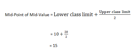
5. Mid – point or Mid – Value – It is the central point of a class – interval. It is calculated by dividing the total of magnitude of lower and upper limits by 2. For example – mid – point of class 10 – 20 will be:

6. Frequency – It refers to number of times a given value appears in a distribution. For example – suppose there are 20 students in a class and out of them, 9 students have got marks between 60-70, 6 got between 70 – 80 marks, and 5 got between 80 – 90 marks. Now frequencies will be 9, 6 and 5 respectively.

Types of Continuous Series

The continuous series are mainly of following types:

1. Exclusive series
2. Inclusive Series
3. Open-End Distribution
4. Cumulative Frequency Series (Less than and More than)
5. Unequal class-interval series
6. Mid-value series.

1. Exclusive Series – Exclusive Series is the series in which upper limit of one class becomes the lower limit of the next class. Such classification ensures continuity of data. For example – if lower limit is 10 and its upper limit is 20, then the class will be 10-20. It includes all values more than or equal to 10 but less than 20. The value 20 and above will go into the next class (20-30).

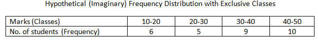
• In the given example, a student with marks between 10 & 19.9 will come in 10-20 class.
• A student whose mark is 20 would be included in the class 20-30.

2. Inclusive Series – Inclusive Series is the series in which both lower and upper limits of a class-interval are included in the interval itself. Thus, under this series, overlapping of intervals is avoided. For example – if lower limit is 10 and its upper limit is 19, then this class will be 10-19. It will include all times more than or equal to 10 and less than or equal to 19.

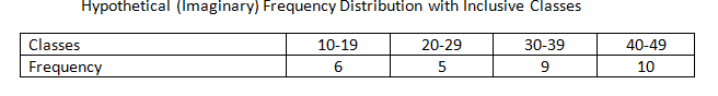
In the given example, a student getting 29 marks will be included in 20- 29 class-interval and similarly a student getting 39 marks is included in 30-39 class-interval.

3. Open – End Distribution – In a frequency distribution, if the lower limit of the first class and the upper limit of last class is not given, it is known as open-end distribution.

• In this series, in place of lower limit of first class, words like ‘below’ or ‘less than’ are written; and
• In the last class, in place of upper limit, words like ‘over’, ‘above’ or ‘more than’ are written.
• Example – the given example is of n open-end distribution as lower limit of the first class and upper limit of the last class is not given.

4. Cumulative Frequency Series (‘Less than’ and ‘More than’) – A simple frequency distribution shows how many observations fall in each class. However, if we are interested in knowing the total number of observations getting a value ‘less than’ or ‘more than’ of a particular value of the class, then such simple frequency table fails to furnish the information. This information can be obtained very conveniently with the help of ‘cumulative frequency distribution’.

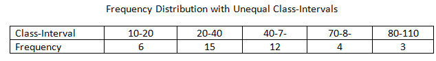
5. Unequal Class-interval Series – When the class-intervals of a frequency distribut8ion are not equal, it is called unequal class-interval series. It happens when data is grouped in a way that some classes cover a larger range and some a smaller range, usually to simplify the presentation of data or to handle extreme values. It is shown in the following table:

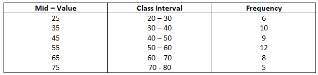
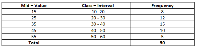
6. Mid – value Series – Mid – Value or Mid-point is the middle value of a class-interval. When such mid-values are given, it is called mid-value series.

Steps to convert Mid-value Series to Continuous Series

• Step 1 – First of all, calculate the difference between the two mid-values.
• Step 2 – Then, half of the difference is subtracted and added to each mid-value to find the lower and upper limits respectively of the class-intervals.

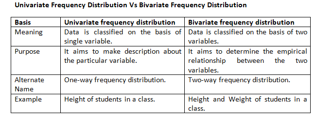
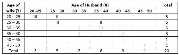
Bivariate Frequency Distribution – When the data is classified on the basis of two variables, the distributions is known as Bivariate frequency distribution or Two – way frequency distribution.

• In this method, values of each variable are grouped into classes, just like in univariate distributions.
• If one variable has m classes and the other has n classes, the bivariate frequency table will have m x n cells.

Unsolved Practical’s

Individual Series

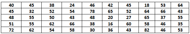
1. Following are the figures of marks obtained by 40 students. You are required to arrange them in ascending and in descending order.

Solution –

Ascending order (Smallest to the larges) = 3, 3, 4, 5, 6, 6, 7, 8, 8, j8, 9, 10, 10, 10, 10, 11, 11, 12, 13, 14, 14, 14, 14, 15, 16, 17, 17, 18, 18, 18, 18, 19, 19, 21, 22, 22, 25

Descending order largest to smallest = 25, 22, 22, 21, 19, 19, 18, 18, 18, 18, 17, 17, 16, 16, 15, 15,  14, 14, 14, 14, 13, 12, 11, 11, 10, 10, 10, 10, 9, 8, 8, 8, 7, 6, 6, 5, 4, 3, 3

Discrete Series

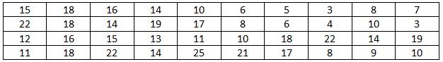
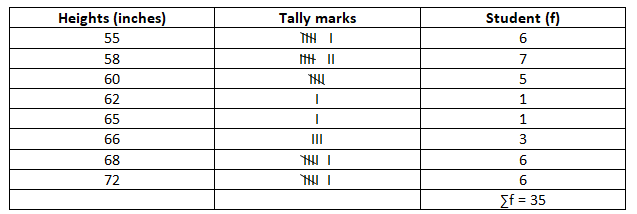
2. Heights (in inches) of 35 students of a class in given below. Classify the following data in a discrete frequency series.

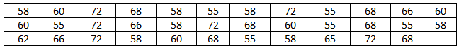
Solution –

Continuous Series

Exclusive Series

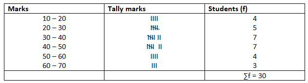
3. The following are the marks of the 30 students in Statistics. Prepare a frequency distribution taking the class-intervals as 10-20, 20-30 and so on.

Solution –

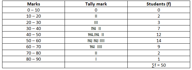
4. Following are the marks (out of 100) obtained by 50 students in statistics:

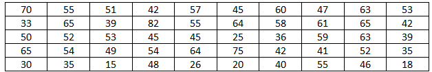
Solution –

Inclusive Series

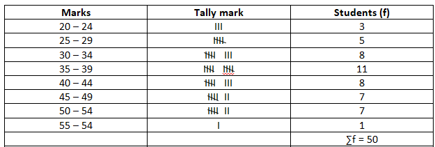
5. Prepare a frequency distribution taking class-intervals 20-24, 25-29, 30-34 and so on, from the following data:

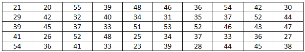
Solution –

Open-end Distribution

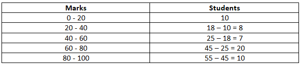
6. Form the following data, calculate the lower limit of the first class and upper limit of the last class.

Solution –

Lower limit = 420 – 20

                   = 400

Upper limit = 480 + 20

                   = 500

7. Calculate the missing class-intervals from the following distribution:

Solution –

50 – 20 = 30

90 – 50 = 40

140 – 90 = 50

Missing

The missing has class intervals with different size. Because of that, the missing class interval cannot be found

Cumulative Frequency Series

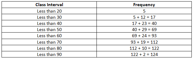
8. Convert the following ‘more that’ cumulative frequency distribution into a ‘less than’ cumulative frequency distribution.

Solution –

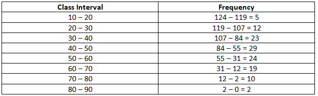
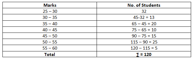
9. Convert the following cumulative frequency series into simple frequency series.

Solution –

Mid-value Series

10. Prepare a frequency distribution from the following data:

Solution –

35 – 25 = 10

10 / 2 = 5

Lower limit = -5

Upper limit = +5

25 – 5 = 20 lower

25 + 5 = 30 lower

Bivariate Frequency Distribution

11. The ages of 20 husbands and wives are given below. Form a two-way frequency distribution showing the relationship between the ages of husbands and wives with the class-intervals 20-25, 25-30, etc.

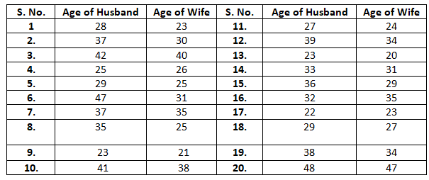
Solution –

Miscellaneous Questions

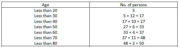
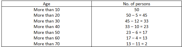
12. From the following data of the ages of different people, prepare less than and more than cumulate frequency distribution.

Solution –

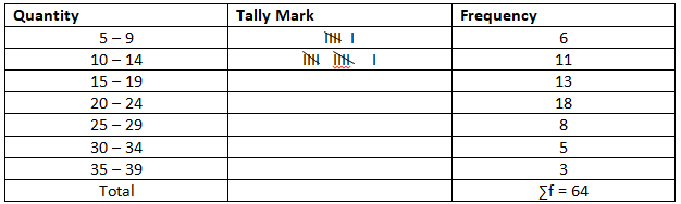
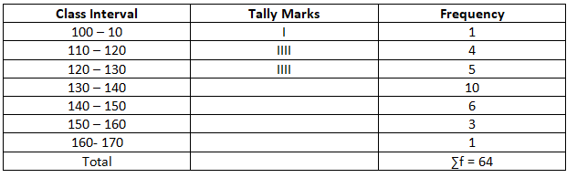
13. In a survey, it was found that 64 families bought milk in the following quantities in a particular month. Prepare a frequency distribution with classes as 5-9, 10-14 etc.

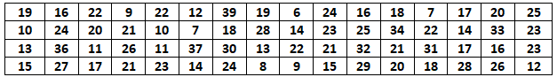
Solution –

14. You are given below a mid value series, convert it into a continuous series.

Solution –

15. For the data given below, prepare a frequency distribution table with classes 100-110, 110-120, etc.

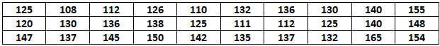
Solution –

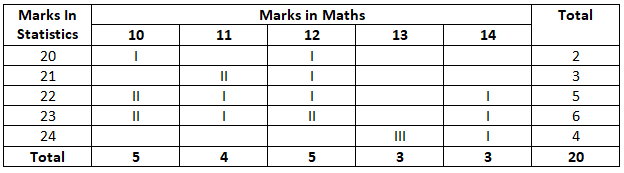
16. Prepare a bivariate frequency distribution for the following data for 20 students:

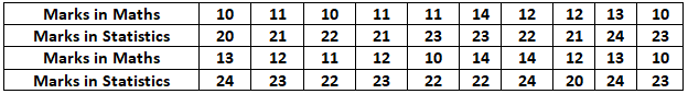
Solution –

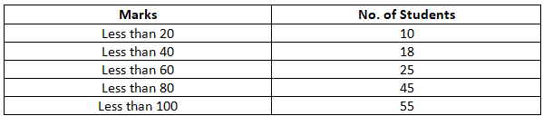
17. In a school, no student has scored less than 25 marks or more than 60 marks in an examination. Their cumulative frequencies are as follows:

Solution –

18. Marks scored by 50 students are given below:

• Arrange the marks in ascending order.
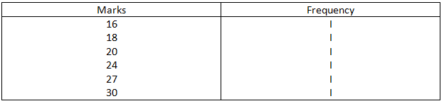
• Represent the marks in the form of discrete series.
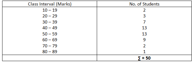
• Construct an inclusive frequency distribution with first class as 10-19. Aslo construct class boundaries.
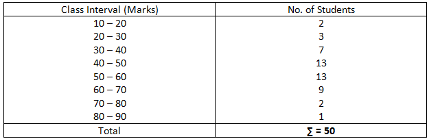
• Construct a frequency distribution with exclusive class-intervals, taking the lowest class as 10-20.
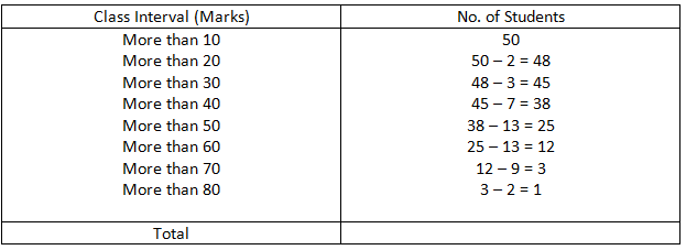
• Convert the exclusive series constructed in (d) into ‘less than’ and ‘more than’ cumulative frequency distribution.

Solution –

1. Arranging in Ascending order –

16, 18, 20, 24, 27, 30, 32, 35, 36, 37, 38, 38, 40, 42, 43, 43, 43, 45, 45, 45, 46, 46, 46, 48, 48, 50, 51, 52, 52, 53, 53, 54, 54, 55, 55, 55, 58, 58, 60, 62, 62, 64, 64, 65, 65, 66, 66, 72, 78, 82.