Consumer’s Equilibrium

INTRODUCTION

A consumer is the main decision-maker of consumption pattern. A consumer is one who buys goods and services for satisfaction of wants. The consumer makes decision with regard to the kind of goods to be purchased in order to satisfy their wants. The main objective to get maximum satisfaction from spending the income on various goods and services.

A consumer has to follow some principles or laws in order to attain the highest satisfaction level. The two main approaches to study consumer’s behavior and consumer’s equilibrium are:

1. Cardinal Utility Approach (or Marshall’s Utility Analysis or Marginal Utility Analysis)
2. Ordinal Utility Approach (or Indifference Curve Analysis or Hicksian Analysis)

Cardinal Utility Approach – People consume different goods and services in order to maximize their satisfaction level. However, to do this, it is necessary to determine the quantum of satisfaction obtained from a particular commodity. Under the Cardinal Utility Approach, the concept of “Utility” is used to attain the Consumers’ Equilibrium.

Concept of Utility – Although the concepts of ‘taste’ and ‘satisfaction’ are familiar to all of us, it is much more difficult to express these concept in concrete terms. For example – Suppose you have just eaten an ice cream and a piece of chocolate. Can you tell how much you are satisfied from each of these items? You can probably tell which item you like more. But, it is very difficult to express measure of satisfaction. Due to this reason, economists developed the concept of utility.

Meaning of Utility – Utility refers to want satisfying power of a commodity. It is the satisfaction, actual or expected, derived from the consumption of a commodity. Utility differs from person-to-person, place-to-place and time-to-time. In the words of Prof. Hobson, “Utility is the ability of a good to satisfy a want”.

How to Measure Utility? – After understanding the meaning of utility, the next big question is: How to measure utility? According to classical economical, utility can be measured, in the same way, as weight or height is measured. For this, economists assumed that utility can be measured in cardinal (numerical) terms.

Example – Measurement of satisfaction in utils – Suppose you have just eaten an ice cream and a chocolate. You agree to assign 20 units as utility derived from the ice cream. Now the question is: how many utils be assigned to the chocolate? If you liked the chocolate less, then you may assign utils less than 20. However, if you liked it more, you would give it a number greater than 20. Suppose, you assign 10 utils to the chocolate, then it can be concluded that you liked the ice cream twice as much as you liked the chocolate.

Total Utility (TU) – Total utility refers to the total satisfaction obtained from the consumption of all possible units of a commodity. It measures the total satisfaction obtained from the consumption of all the units of that good.

For example – if the 1^st ice cream gives you a satisfaction of 20 utils and 2^nd one gives 16 utils, then TU from 2 ice cream is 20 + 16 = 36 utils. If the 3^rd ice cream generates satisfaction of 10 units, then TU from 3 ice cream will be 20 + 16 + 10 = 46 utiles.

TU can be calculate as:

TU_n = U₁ + U₂ + U₃ + ………………. + U_n

Where:

TU_n = total utility from n units of a given commodity

U₁ , U₂ , U₃ , ……………….  U_n = Utility from the 1^st , 2^nd , 3^rd ………….., n^th unit

N = Number of units consumed

Marginal Utility (MU) – Marginal utility is the additional derived from the consumption of one more unit of the given commodity. It is the utility derived from the last unit of a commodity purchased. As per the given example, when 3^rd ice cream is consumed, TU increases from 36 utils to 46 utils. The additional 10 utils from the 3^rd ice cream is the MU. In the words of Chapman, “Marginal utility is an addition made to the utility by consuming one more unit of a commodity”.

MU can be calculated as: MU_n = YU_n = TU_n-1

One More way to calculate MU – MU is the change in TU when one more unit is consumed. However, when a change in units consumed is more than one, then MU can also be calculate as:

                  MU = Change in Total Utility / Change in number of Units

                          = ΔTU / ΔQ

Relationship between TU and MU

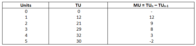
1. TU increase with an increase in consumption of a commodity as long as MU is positive, i.e. till the 4^th ice cream. In this phase, TU increases, but a diminishing rate as MU from each successive unit tends to diminish.
2. When TU reaches its maximum, MU becomes zero, i.e. when the 5^th ice cream is consumed. This is known as point of satiety. TU curve stops rising at the stage.
3. When consumption is increased beyond the point of satiety, TU starts fallings as MU becomes negative.

Law of Diminishing Marginal Utility

Law of diminishing marginal utility (DMU) states that as we consume more and more units of a commodity, the utility derived from each successive unit goes on decreasing. In making choices, most people spread their incomes over different kinds of goods. People prefer a variety of goods because consuming more and more of any one good reduces the marginal satisfaction derived from further consumption of the same good. This law expresses an important relationship between utility and the quantity consumed of a commodity. Let us understand this law with the help of an example:

Assumptions of Law of Diminishing Marginal Utility

The law of DMU operates under certain specific conditions. Economists call them the ‘assumptions’ of this law. These are as follows:

1. Cardinal measurement of utility – It is assumed that utility can be measured and consumer can express his satisfaction in quantitative terms such as 1,2,3 etc.
2. Monetary measurement of utility – It is assumed that utility is measurable in monetary terms.
3. Consumption of reasonable quantity – it is assumed that a reasonable quantity of the commodity is consumed. For example – we should compare the MU of a glassful of water and not of a spoonful of water. If a thirsty person is given water in a spoon, then every additional spoon will yield him more utility. So, to hold the law true, a suitable and proper quantity of the commodity should be consumed.
4. Continuous consumption – It is assumed that consumption is a continuous process For example – if one ice cream is consumed in the morning and another in the evening, then the second ice cream may provide equal or higher satisfaction as compared to the first one.
5. No change in Quality – Quality of the commodity consumed is assumed to be uniform. A second cup of ice cream with nuts and toppings may give more satisfaction than the first one, if the first ice cream was without nuts or toppings.
6. Rational consumer – the consumer is assumed to be rational who measures, calculates and compares the utilities of different commodities and to maximize total satisfaction.

Consumer’s Equilibrium – The term ‘equilibrium’ is frequently used in economic analysis. Equilibrium means a state of rest or a position of  no change. It refers to a position of rest, which provides the maximum benefit or gain under a given situation. A consumer is said to be in equilibrium, when he does not intend to change his level of consumption, i.e., when he derives maximum satisfaction.

            Consumer’s Equilibrium refers to the situation when a consumer is having maximum satisfaction with limited income and has no tendency to change his way of existing expenditure.

Consumer’s equilibrium can be discussed under two different situations:

1. Consumer spends his entire income on a Single Commodity
2. Consumer spends his entire income on Two Commodities

Consumer’s Equilibrium in case of Single Commodity – The law of DMU can be used to explain consumer’s equilibrium in the case of a single commodity. Therefore, all the assumptions of the Law of DMU are taken as assumptions of consumer’s equilibrium in the case of a single commodity. A consumer purchasing a single commodity will be at equilibrium, when he is buying such a quantity of that commodity, which gives him maximum satisfaction. The number of units to be consumed of the given commodity by a consumer depends on 2 factors:

1. Price of the given commodity;
2. Expected utility (Marginal Utility) from each successive unit.

Marginal Utility in terms of Money = Marginal Utility in utils / Marginal Utility of one rupee (MU_M)

Equilibrium Condition – Consumer in consumption of single commodity (say, x) will be at equilibrium when:

Marginal Utility (MU_x) is equal to Price (P_x) paid for the commodity; i.e. MU_x = P_x

Consumer’s Equilibrium in case of Two Commodities – The Law of DMU applies in case of either once commodity or one use of a commodity However, in real life, a consumer normally consume more than one commodity. In such a situation, ‘Law of Equi-Marginal Utility’ helps in optimum allocation of his income.

As the law of Equi-marginal utility is based on law of DMU, all assumption of the latter also apply to the former. Let us now discuss equilibrium of consumer by taking tow goods; ‘x’ and ‘Y’. The same analysis can be extended for any number of goods. In the case of consumer equilibrium under a single commodity, we assumed that the entire income was spent on a single commodity. Now, the consumer wants to allocate his money income between the two goods to attain the equilibrium position.

According to the low of Equi-marginal utility, a consumer gets maximum satisfaction, when the ration of MU of two commodities and their respective prices are equal and MU falls as consumption increases. It means, there are two necessary condition to attain Consumer’s Equilibrium in case of Two Commodities:

1. The ratio of Marginal Utility to Price is same in case of both the goods.

• We know, a consumer in consumption of single commodity (say, x) is at equilibrium

When = MUx / Px

           = MUm

• Similarly, consumer consuming another commodity (say, y) will be at equilibrium when = MUy / Py

                              = MUm

Equating 1 and 2, we get: MUx / Px = MUy / Py = Mum

As marginal utility of money (MUm) is assumed to be constant, the above equilibrium condition can be restated as:

MUx / Px = MUy / Py   Or     MUx / MUy = Px / Py

When Px = Py then the equilibrium condition can be restated as: MUx = MUy.

2. MU  falls as consumption increases : The second condition needed to attain consumer’s equilibrium is that MU of a commodity must fall as more of it is consumed. If MU does not fall as consumption increases, the consumer will end up buying only one good which is unrealistic and consumer will never reach the equilibrium position.

Ordinal Utility Approach (Indifference Curve Or Hicksian Analysis)

Modern economists disregarded the concept of ‘cardinal measure of utility’. They were of the opinion that utility is a psychological phenomenon and that it is next to impossible to measure utility in absolute terms. According to them, a consumer can rank various combinations of goods and services in order of his preference. For example – if a consumer consumes two goods, apples and Bananas, then he can indicate:

1. Whether he prefers apple over banana; or
2. Whether he prefers banana over apple; or
3. Whether he is indifferent between apples and bananas, i.e. both are equally preferable and both of them give him same level of satisfaction.

Meaning of Indifference Curve – When a consumer consumes various goods and services, then the there are some combinations, which give him exactly the same total satisfaction. The graphical representation of such combination is termed as indifference curve. Indifference curve refers to the graphical representation of various alternative combinations of bundles of two goods among which the consumer is indifferent. Alternately, indifference curve is a lacus of points that shows such combinations of two commodities which give the consumer same satisfaction. An indifference curve is also known as ‘equal satisfaction curve’ or ‘Iso-utility curve’.

Indifference Map – Indifference Map refers to the family of indifference curves that represent consumer preferences over all the bundles of the two goods.

An indifference curve represents all the combinations, which provide same level of satisfaction. However, every higher or lower level of satisfaction can be shown on different indifference curves. It means, infinite number of indifference curves can be drawn. IC₁ represents the lowest satisfaction, IC₂ shows satisfaction more than that of IC₁ and the highest level of satisfaction is depicted by indifferent curve IC₃. However, each indifference curve shows the same level of satisfaction individually.

Marginal Rate of Substitution (MRS)

MRS refers to the rate at which the commodities can be substituted with each other, so that total satisfaction of the consumer remains the same. For example, in the example of apples (A) and bananas (B), MRS of ‘A’ for ‘B’, will be number of units of ‘B’, that the consumer is willing to sacrifice for an additional unit of ‘A’, so as to maintain the same level of satisfaction.

MRS_AB = Units of Bananas (B) willing to Sacrifice / Units of Apples (A) willing to gain

MRS_AB = ΔB / ΔA

MRS_AB is the rate at which a consumer is willing to give up Bananas for one more unit of Apple. It means, MRS measures the slope of indifference curve.

Assumptions of Indifference Curve

The various assumption of indifference curve are:

1. Two commodities – It is assumed that the consumer has a fixed amount of money, the whole of which is to be spent on the two goods, given the constant prices of both goods.
2. Non Satiety – It is assumed that the consumer has not reached the point of saturation. A consumer always prefers more of both commodities, i.e. he always tries to move to a higher indifference curve to get higher and higher satisfaction. The consumer’s choice is presumed to be monotonic, i.e. a consumer always prefers a bundle with more goods as it offers him a higher level of satisfaction.
3. Ordinal Utility – A consumer can rank his preferences on the basis of the satisfaction from each bundle or goods.
4. Diminishing marginal rate of substitution – Indifference curve analysis assumes diminishing marginal rate of substitution. Due to this assumption, an indifference curve is convex to the origin.
5. Rational Consumer – The consumer is assumed to behave in a rational manner, i.e. he aims to maximize his total satisfaction.

Properties of Indifference Curve –

1. Indifference curves are always convex to the origin – An indifference curve is convex to the origin because of diminishing MRS. MRS declines continuously because of the law of diminishing marginal utility. When the consumer consumers more and more apples, his marginal utility from apples keeps on declining and he is willing to give up less and less of bananas for each apple. Therefor, indifference curve are convex to the origin. It must be noted that MRS indicates the slope of indifference curve.
2. Indifference curve slope down wards – It implies that as a consumer consumes more of one good, he must consume less of the other good. This happens because if the consumer decides to have more units of one good (say apples), he will have to reduce the number of units of another good (say bananas), so that total satisfaction remains the same.
3. Higher Indifference curves represent higher levels of satisfaction – A higher indifference curve represents a large bundle of goods, which means more utility because of monotonic preference. Consider point ‘A’ on IC₁. At ‘A’ consumer gets the combination (OR, OP) of the two commodities x and y. At ‘B’, consumer gets the combination (OS, OP). As OS > OR, the consumer gets more satisfaction at IC₂.
4. Indifference curves can never intersect each other – As two indifference curves cannot represent the same level of satisfaction, they cannot intersect each other. It means, only one indifference curve will pass through a given point on an indifference map.

Budget Line

So far, we have discussed different combinations of two goods that provide same level of satisfaction. But, which combination a consumer actually purchases depends upon his income (‘consumer budget) and prices of the two commodities. Consumer Budget states the real income or purchase power of the consumer from which he can purchase certain quantitative bundles of two goods as a given price. It means, a consumer can purchase only those combination (bundles) of goods, which cost less than or equal to his income.

Budget line is a graphical representation of all possible combinations of two goods which can be purchased with given income and prices, such that the cost of each of these combinations is equal to the monetary income of the consumer. Alternately, Budget Line is the locus of different combinations of the two goods which the consumer consumes and which cost exactly his income. Budget Line is also known as: (A) Price Line; (b) Price Opportunity Line; (c) Price-Income Line; or (d) Budget Constraint Line.

Budget Set – Budget set is the set of all possible combination of the two goods which a consumer can afford given his income and prices in the market. In addition to the three options, there are some more options available to the consumer his income, even if entire income is not spent. Budget set includes all the bundles with a total income of Rs.20, i.e. possible bundles or consumer’s bundles are: (0, 0); (0, 1); (0, 2); (1, 0); (2, 0); (1, 1). Consumer’s Bundle is a quantitative combination of two goods which can be purchased by a consumer from his given income.

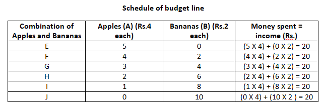
Diagrammatic Explanation of Budget Line – Suppose, a consumer has a budget of Rs.20 to be spent on two commodities: apples (A) and bananas (B). If apple is priced at Rs.4 each and banana at Rs.2 each, then the consumer can determine the various combination (bundles), which form the budget line. The possible option for spending income of Rs.20.

Algebraic Expression of Budget Line

The budget line can be expressed as an equation:

            M = (P_A X Q_A) + (P_B X Q_B)

Where:

M = Money income;

Q_A= Quantity of apples (A);

Q_B  = Quantity of bananas (B);

P_A  = Price of each Apple;

P_B = Price of each bananas.

All points on the budget line ‘AB’ indicate those bundles, which cost exactly equal to ‘M’.

Slope of the Budget Line – We know that the slope of a curve is calculated as a change in variable on the vertical Y-axis divided by a change in variable on the horizontal or X-axis. In the example of apples and bananas, slope of the budget line will be number of units of bananas, that the consumer is willing to sacrifice for an additional unit of apple.

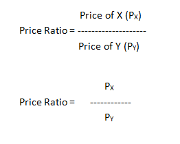
Price Ratio – Price Ratio is the price of the good on the horizontal or X-axis divided by the price of the good on the vertical or Y-axis. For instance, if good X is plotted on the horizontal axis and good Y on the vertical axis, then:

Properties of Budget Line

The two main properties of Budget line are:

1. Budget Line is Downward Sloping – Budget line has a negative slope, i.e. it slopes downwards as more of one good can be bought by decreasing some units of the other good.
2. Budget Line is a straight line – The slope of Budget line is represented by the Price Ratio. As Price Ratio is constant throughout, the budget line is a straight line.

Shift in Budget line

Budget line is drawn with the assumptions of constant income of consumer and constant prices of the commodities. A new budget line would have to be drawn if either (a) Income of the consumer changes, or (b) Price of the commodity changes.

1. Effect of a Change in the Income of Consumer – If there is any change in the income, assuming no change in the price of a apples and bananas, then the budget line will shift. When income increases, the consumer will be able to buy more bundles of goods, which was previously not possible.
2. Effect of change in Price (Apple and Bananas) – If there is any change in price of two commodities, assuming no change in money income of consumer, then budget line will change.

• Change in Price of both commodities
• Change in the Price of commodities on X-axis (Apples)
• Change in the Price of commodity on Y-axis (Bananas)

Consumer’s Equilibrium by Indifference curve Analysis

Consumer equilibrium refers to a situation, in which a consumer derives maximum satisfaction, with no intention to change it and subject to given prices and his given income. The point of maximum satisfaction is achieved by studying the indifference map and budget  line together.

Conditions of Consumer’s Equilibrium – The consumer’s equilibrium under the indifference curve theory must meet the following two conditions:

• MRS_XY = Ratio of Prices or P_x/P_Y = Market Rate of Exchange (MRE)

• MRS continuously falls – The second condition for consumer’s equilibrium is that MRS must be diminishing at the point of equilibrium, i.e. the indifference curve must be convex to the origin at the point of equilibrium. Unless MRS continuously falls, the equilibrium cannot be established.

Cardinal Utility V_s Ordinal Utility

1. Under Cardinal Utility Approach, it is assumed that utility can be measured in cardinal terms, such as 1,2,3, etc. However, according to the Ordinal Utility Approach, Utility is a subjective concept, which cannot be measured and we can just rank the scale of preferences.
2. Under the Cardinal Approach, the term “util” was developed as a unit to measure utility, whereas, no such unit of measurement was developed under Ordinal Approach.
3. Example – Suppose a person consumes apple and banana.

• According to Cardinal Approach, the consumer can assign utils to both commodities, say, 20 utils to apple and 15 utils to banana. This signifies that apple offers 5 more utils than banana.
• According to Ordinal Approach, the consumer cannot express the satisfaction in exact terms. It means, if the consumer likes apple more than banana, then the he will give 1^st rank to apple and 2^nd rank to banana.

UNSOLVED PRACTICLA

Practical’s on TU and MU

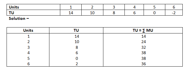
1. A person’s total utility (TU) schedule is given below. Derive marginal utility (MU).

Solution –

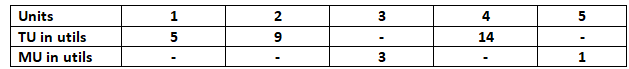
2. Derive MU from the total utility (TU) schedule given below:

Solution –

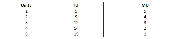
3. A person’s MU schedule is given below. Derive TU:

4. Calculate the missing figures.

Solution –

Practical’s on Consumer’s Equilibrium (Single Commodity)

5. Suppose price of a commodity ‘x’ is given as Rs.5 and the MU (in terms of money) for 4 units is given as:

How many units should a consumer purchase, so that his satisfaction is maximum?

Solution –

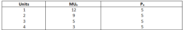
According to consumer’s equilibrium a consumer attains maximum satisfaction when MU_x becomes equal to P_x.

So, according to the question, a consumer attains maximum satisfaction when he consumer 3 units of good.

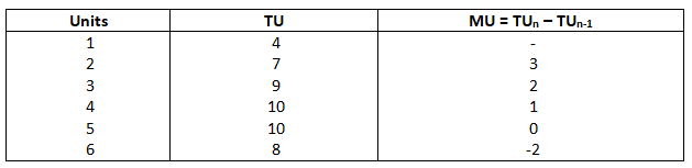
6. Following is the utility schedule of a consumer:

If the commodity is sold for Rs.5 and MU of one rupee is 2 utils. How many units will a consumer purchase to maximize his satisfaction?

Solution –

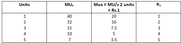
When a consumer is consuming 4 units of a product, he will get maximum satisfaction as at that point Mux is equal to Px.

Practicals on Consumer’s Equilibrium (Two Commodities)When a consumer is consuming 4 units of a product, he will get maximum satisfaction as at that point Mux is equal to Px.

Practicals on Consumer’s Equilibrium (Two Commodities)When a consumer is consuming 4 units of a product, he will get maximum satisfaction as at that point Mux is equal to Px.

Practicals on Consumer’s Equilibrium (Two Commodities)

7. The MU schedule for goods X and Y are given. Price of both the goods is Rs.1 each and the income of Ramesh (an individual) is assumed to be Rs.5. Determine, how many units of both the commodities should be purchased by Ramesh to maximize his total utility. What is the total amount of utility received by Ramesh at the point of equilibrium?

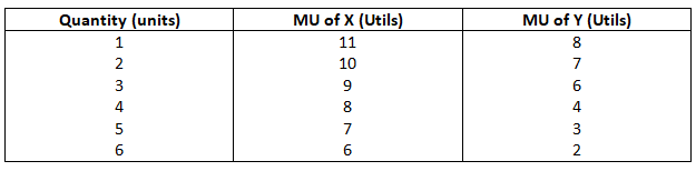
Solution – A consumer consuming two goods will be at equilibrium when.

Mu_x / Px = Mu_y / P_Y

MU falls as consumption increases

A consumer will get maximum satisfaction when he consumes: –

4 units of good X and 1 unit of, good Y.

• Total utility = 11 + 10 + 9 + 8 + 8
•                    = 46 utils.

8. The marginal utility schedule for goods A and B are given. Price of both the goods is Rs.1 each and the income of Ms. Nidhi is assumed to be Rs.8. Determine, how many units of both the commodities should be purchased by Nidhi to maximize her total utility. Also, calculate the total utility at the point of equilibrium.

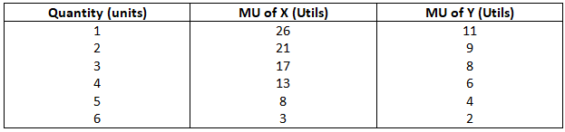
Solution –

Ms Nidhi will be at equilibrium when she is consuming –

5 units of good A and 3 units of good B

Total utility = 26 + 21 + 17 + 13 + 8 + 11 + 9 + 8 = 113 utils.

9. Suppose consumer can buy 5 units of good x and 4 units of good y, if he spends his entire income. The price of good x is Rs.10 and that of y is Rs.12. Calculate the income of the Consumer.

Solution –

To find : – Income of a consumer

He buys : –

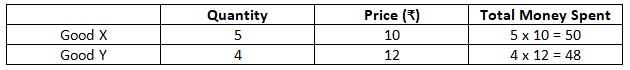
So, income of a consumer = 50 + 48

                                           = Rs.98

10. Amit wants to purchase two goods which are available in integer units only. If his income is Rs.40 and both the goods are priced at Rs.10 each, then write the bundles which cost exactly Rs.40.

Solution –

Let the 2 goods be A and B.

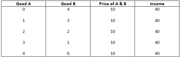
Bundles of (A, B) = (0, 4) (1, 3) (2, 2) (3, 1) (4, 0)

11. Suppose there are three bundles containing good 1 and good 2: Bundle (10, 10); Bundle (10, 9) and Bundle (7, 10). Which bundle will be preferred by the consumer, if he has monotonic preferences?

Solution –

Bundle (10,10) will be preferred by a consumer if he has Monotonic preference because this bundle contains more of both the Goods.

12. Manish is indifferent to the bundles (4, 7) and (4, 8). Indicat, whether Manish has monotonic preference or not?

Solution –

No, Manish did not have monotonic preference because if he had monotonic preference then he would have preferred bundle (4, 8) as it contains more of one good.